Importa le librerie
import numpy as np
import pandas as pd
Carica il file dei dati
data=pd.read_csv("president_heights.csv")
Dai un’occhiata
print(data)


    order              name height(cm)
 0      1 George Washington        189
 1      2        John Adams        170
 2      3  Thomas Jefferson        189
 3      4     James Madison        163
 4      5      James Monroe        183
..    ..                ...        ...
37     40     Ronald Reagan        185
38     41 George H. W. Bush        188
39     42      Bill Clinton        188
40     43    George W. Bush        182
41     44      Barack Obama        185
Estrai le altezze
heights=np.array(data["height(cm)"])
print(heights)

[189 170 189 163 183 171 185 168 173 183 173 173 175 178 183 193 178 173
 174 183 183 168 170 178 182 180 183 178 182 188 175 179 183 193 182 183
 177 185 188 188 182 185]
Informazioni statistiche
print("Altezza minima     :", heights.min())
print("Altezza media      :", heights.mean())
print("Altezza massima    :", heights.max())
print("Deviazione standard:", heights.std())

Altezza minima     : 163
Altezza media      : 179.73809523809524
Altezza massima    : 193
Deviazione standard: 6.931843442745892
Ancora…
print("Primo quartile (25%):", np.percentile(heights, 25))
print("Mediana             :", np.median(heights)        )
print("Terzo quartile (75%):", np.percentile(heights, 75))

Primo quartile (25%): 174.25
Mediana             : 182.0
Terzo quartile (75%): 183.0
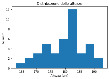
Grafici
import matplotlib.pyplot as plt

plt.hist(heights)
plt.title('Distribuzione delle altezze')
plt.xlabel('Altezza (cm)')
plt.ylabel('Numero');

plt.show()
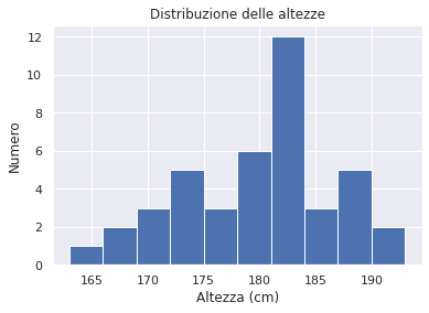
Aggiungi le impostazioni grafiche di seaborn
import matplotlib.pyplot as plt
import seaborn           as snc

snc.set()

plt.hist(heights)
plt.title('Distribuzione delle altezze')
plt.xlabel('Altezza (cm)')
plt.ylabel('Numero');

plt.show()
Vedi: https://jakevdp.github.io/PythonDataScienceHandbook/02.04-computation-on-arrays-aggregates.html